
Speed-Fuel Curve
How to run this?
Go here to instantly run all code below inside of your browser.
Use case
In the basics use case we demonstrated how to simulate a ship's performance in a single condition at a single speed.
We will extend this example and simulate a ship's performance over multiple speeds. This will allow us to construct a speed-fuel table and speed-fuel curve, showing the required fuel consumption for each speed of the ship.
Authorize
Let's first make sure we're authorized to use the API by running the following code.
If everything is alright, you should see a list of ships.
import json
import requests

API_URL = "https://api.toqua.ai"

url = "https://api.toqua.ai/ships/"
headers = {"accept": "application/json", "X-API-Key": API_KEY}
response = requests.get(url, headers=headers)

print(json.dumps(response.json(), indent=2))
[
  {
    "name": "Demo Vessel",
    "imo_number": 9999999,
    "type": "Tanker",
    "country": "SC",
    "build_year": 2015,
    "shipyard": "Toqua Shipyard",
    "dwt": 220000.0,
    "beam": 55.0,
    "loa": 300.0,
    "mcr": 21900.0,
    "max_rpm": 60.0,
    "uuid": "eycrYbrzJNsJecGqKraUCn"
  }
]
Fill in the IMO number of the ship you want to analyze.
IMO_NUMBER = 9999999Conditioning parameters
Let's again define our conditions.
wind_speed = 6          # [m/s]
wind_direction = 180    # [degrees]
wave_height = 2         # [m]
wave_direction = 90     # [degrees]
current_speed = 0.5     # [m/s]
current_direction = 0   # [degrees]
mean_draft = 20         # [m]
trim = -1               # [m]
ship_heading = 0        # [degrees]
fuel_specific_energy  = 41.5 # [MJ/kg]
Our entrypoint will this time be a list, rather than a single value. We will analyze the ship's fuel consumption in speeds ranging from a STW of 8 knots to 16 knots.
stw = list(range(8, 17))

print(stw)
[8, 9, 10, 11, 12, 13, 14, 15, 16]Define the API input
Remember that the Toqua API expects the model input to look like this:
{
     "date": "...",
     "data": {
          "stw": [...],
          "draft_avg": [...],
          "trim": [...],
          "wave_direction": [...],
          "wave_height": [...],
          "wave_period": [...],
          "current_speed": [...],
          "current_direction": [...],
          "wind_direction": [...],
          "wind_speed": [...],
          "ship_heading": [...],
          "fuel_specific_energy": [...]
     }
}
We will again ignore the date parameter for now.
Each parameter expects a list of values and all lists must have exactly the same length.
The parameter value at each index $i$ corresponds to $$Condition_i = {stw_i, wave_direction_i, wave_speed_i, draft_avg_i, ...}$$
Only the stw parameter is currently a list and we are only simulating a single condition, so we will have to duplicate the conditioning parameters once for each element in the stw list.
length_input = len(stw)

api_input = {
    "data": {
        "stw": stw,
        "wave_direction": [wave_direction]*length_input,
        "wave_height": [wave_height]*length_input,
        "wind_direction": [wind_direction]*length_input,
        "wind_speed": [wind_speed]*length_input,
        "current_direction": [current_direction]*length_input,
        "current_speed": [current_speed]*length_input,
        "draft_avg": [mean_draft]*length_input,
        "trim": [trim]*length_input,
        "ship_heading": [ship_heading]*length_input,
        "fuel_specific_energy": [fuel_specific_energy]*length_input
    }
}
Query the API
def query_api(imo_number, payload):
    url = f"https://api.toqua.ai/ships/{imo_number}/models/latest/predict"
    headers = {
        "accept": "application/json",
        "content-type": "application/json",
        "X-API-Key": API_KEY,
    }
    response = requests.post(url, json=payload, headers=headers)
    return response
Let's look at the values the model predicts.
response = query_api(IMO_NUMBER, api_input)

print(response.json())
{'sog': [7.02808, 8.02808, 9.02808, 10.02808, 11.02808, 12.02808, 13.02808, None, None], 'stw': [8.0, 9.0, 10.0, 11.0, 12.0, 13.0, 14.0, None, None], 'me_rpm': [35.563477161420984, 38.86856315406255, 42.3286138994565, 45.958934292444695, 49.77248238124245, 53.780632616735986, 57.993745359998364, None, None], 'me_power': [4014.487664675082, 5034.96591338081, 6306.250909817854, 7883.151679670297, 9830.679471751078, 12225.665331559763, 15158.644854083537, None, None], 'me_fo_consumption': [18.24386889835794, 22.461921943399787, 27.57687777045103, 33.79875072031291, 41.47119688825557, 51.21728628254814, 64.2267638497258, None, None], 'me_fo_emission': [57.842186342243835, 71.21552352154902, 87.43249097121499, 107.15893915875206, 131.48442973421427, 162.38440615881885, 203.63095478555562, None, None], 'errors': [{'error_code': 'max_mcr_limit_exceeded', 'description': '90% Maximum MCR (19710 kW) exceeded.', 'indices': [8]}, {'error_code': 'max_rpm_limit_exceeded', 'description': 'Maximum RPM (60.0 RPM) exceeded.', 'indices': [7, 8]}]}Speed-Fuel Table
Using the Pandas library we can transform this output into table format to make it easier on the eyes, and for future data transformations.
Let's see if any errors occurred during prediction.
import pandas as pd
output_json = response.json()
errors = output_json['errors']
print(errors)
[{'error_code': 'max_mcr_limit_exceeded', 'description': '90% Maximum MCR (19710 kW) exceeded.', 'indices': [8]}, {'error_code': 'max_rpm_limit_exceeded', 'description': 'Maximum RPM (60.0 RPM) exceeded.', 'indices': [7, 8]}]We can see that on indices 7 and 8 the model failed to predict the fuel consumption. This is because for those conditions the predicted power would be above the ship's MCR or Max RPM.
On these indices, the output will contain null values.
# remove the errors from the output json so pandas can read it
del output_json['errors']
df = pd.DataFrame(output_json)
df| sog | stw | me_rpm | me_power | me_fo_consumption | me_fo_emission | |
|---|---|---|---|---|---|---|
| 0 | 7.02808 | 8.0 | 35.563477 | 4014.487665 | 18.243869 | 57.842186 |
| 1 | 8.02808 | 9.0 | 38.868563 | 5034.965913 | 22.461922 | 71.215524 |
| 2 | 9.02808 | 10.0 | 42.328614 | 6306.250910 | 27.576878 | 87.432491 |
| 3 | 10.02808 | 11.0 | 45.958934 | 7883.151680 | 33.798751 | 107.158939 |
| 4 | 11.02808 | 12.0 | 49.772482 | 9830.679472 | 41.471197 | 131.484430 |
| 5 | 12.02808 | 13.0 | 53.780633 | 12225.665332 | 51.217286 | 162.384406 |
| 6 | 13.02808 | 14.0 | 57.993745 | 15158.644854 | 64.226764 | 203.630955 |
| 7 | NaN | NaN | NaN | NaN | NaN | NaN |
| 8 | NaN | NaN | NaN | NaN | NaN | NaN |
There we have our speed-fuel table. For speeds ranging from 8 to 16 knots it tells us the predicted fuel consumption in the conditions we defined earlier.
Speed-Fuel Curve
Finally, to make things more tangible we can use the Plotly library to visualize our table as a speed-fuel curve.
import plotly.express as px

fig = px.line(df, x="stw", y="me_fo_consumption", title='Speed-Fuel Curve')
fig.update_layout(xaxis_title='Speed Through Water [kn]',
                   yaxis_title='Fuel Consumption [mt/day]')
fig.show()fig.write_image("speed-fuel-curve.png")import plotly.express as px
fig = px.line(df, x="stw", y="me_fo_consumption", title='Speed-Fuel Curve')
fig.update_layout(xaxis_title='Speed Through Water [kn]',
yaxis_title='Fuel Consumption [mt/day]')
fig.show()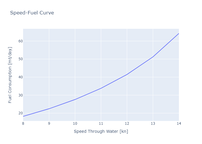
Updated over 1 year ago