
Voyage-Leg Fuel Consumption Breakdown
This use case demonstrates how Toqua's Ship Kernels break down fuel consumption over a voyage leg into key contributing factors (waves, wind, currents, fouling, calm water use, etc.). While this example shows a breakdown over the voyage leg duration using sensor data, similar code can be applied to daily, yearly, or any other time window you want to analyze using either sensor data or noon reports.
Use Case

Notebook Structure
Chapter 1: Data Preparation
- Load Data
- Data Adjustment 1: Remove Obsolete Columns & Add Voyage Column
- Data Adjustment 2: Add Fuel Contributions: Wind, Waves, Current, Draft, and Fuel Quality
- Data Adjustment 3: Add Fuel Contribution: Hull Degradation
- Data Adjustment 4: Apply Fuel Contribution Percentages to Actual Fuel Consumption Rate
- Data Adjustment 5: Convert Daily Fuel Rate (mt/day) to Fuel Consumption
Chapter 2: Visualization
- Data Aggregation
- Select
Voyage_ID- Standard Visual: Voyage-Level Fuel Breakdown
- Advanced Visual: "Daily Fuel Breakdown
- Combined Standard & Advanced Visuals
Toy Example
During a single five-minute logging window the bridge of a VLCC records the values below. These are exactly the inputs the Toqua model needs for a fuel prediction. For this example we assume the ship is sailing in ballast.
| Variable (model field) | Snapshot reading |
|---|---|
| Speed over ground (sog) | 12.7 kn |
| True wind (speed & direction) |
19.4 kn from 200° |
| Wave height & direction | 2 m from 190° |
| Current speed & direction | 1 kn from 20° |
| Draft (draft_avg) | 12.0 m |
| Fuel specific energy (fuel_specific_energy) |
40.0 MJ /kg |
| Measured ME fuel rate | 29 mt /day |
Feeding those raw numbers to the Toqua API returns a fuel rate of 32 mt/day. That is what the model believes the engine should burn under the real conditions.
When we “switch off” one variable at a time, we are building a simple what-if experiment around the model’s baseline prediction of 32 mt/day. Each row in the table shows what happens when a single influence is replaced by its neutral reference value while every other input stays exactly as observed. If the new prediction drops below the baseline (as it does when we remove wind, waves, or ship is empty/laden), that factor is adding fuel; if it rises above the baseline (as with the helping current), the factor was actually saving fuel.
| Factor neutralised | Reference value sent to the API | New model output | Effect on fuel |
|---|---|---|---|
| Wind | Wind speed = 0 kn | 30 mt /day | +2 mt/day (wind costs 2) |
| Waves | Wave height = 0 m | 31 mt /day | +1 mt/day (waves cost 1) |
| Current | Current speed = 0 kn | 34 mt /day | –2 mt/day (current saves 2) |
| Draft | Draft = 8 m (ballast) | 28 mt /day | +4 mt/day (deep draft costs 4) |
| Fuel quality | Fuel = 42.7 mt /day | 31 mt /day | +1 mt/day (poor fuel costs 1) |
The model’s metadata shows the hull is about 10% fouled, which means roughness alone adds roughly two tonnes of fuel per day to the bill.
Once we’ve estimated the model-based impact of each factor, we convert that difference into a percentage relative to the baseline prediction. This percentage is then applied to the vessel’s actual measured fuel rate, translating model behaviour into real-world terms. The result is a consistent, data-grounded estimate of how much each variable contributed to the fuel consumption during that interval.
Because five minutes are 5⁄1440 of a day, each daily quantity shrinks by that factor for an individual log interval. Note that when using noon report data this factor is not required.
Authorize
Let's first make sure we're authorized to use the API. Fill in your API key and run the following code.
If everything is alright, you should see a list of ships.
API_KEY = "your-api-key"import json
import requests
API_URL = "https://api.toqua.ai"
url = "https://api.toqua.ai/ships/"
headers = {"accept": "application/json", "X-API-Key": API_KEY}
response = requests.get(url, headers=headers)
print(json.dumps(response.json(), indent=2))Fill in the IMO number of your ship below
IMO_NUMBER = "your-imo-number"Chapter 1: Data Preparation
Download necessary libraries.
import pandas as pd
from IPython.display import display
from typing import List, Dict, Tuple
import ssl
import json
from urllib.request import Request, urlopen
from urllib.error import HTTPError
import requests
import numpy as np
from tqdm import tqdm
import time
import matplotlib.pyplot as plt
from plotly.subplots import make_subplots
import plotly.graph_objects as go
1.1) Load Data
Load data in CSV format. We're using 5min frequency sensor data, but noon report data can also be used.
df = pd.read_csv("./example_sensor_data.csv")Display first 10 rows.
display(df.head(10))| datetime_end | sog | stw | me_power | me_rpm | me_fo_consumption | heading | trim | sea_depth | operating_mode | ... | wind_wave_height | wind_wave_period | datetime_start_nr | datetime_end_nr | me_fo_consumption_nr | heading_nr | water_displacement | operating_mode_nr | draft_avg | fo_ncv | |
|---|---|---|---|---|---|---|---|---|---|---|---|---|---|---|---|---|---|---|---|---|---|
| 61632 | 2025-01-01 00:00:00+00:00 | 12.7320 | 12.6540 | 15134.1330 | 61.9750 | 76.32 | 89.6430 | 0.5090 | 4084.0 | NaN | ... | 0.360000 | 2.410000 | NaN | 2025-01-01 20:00:00+00:00 | 73.04 | 89.0 | NaN | NaN | 20.3 | 40.2 |
| 61633 | 2025-01-01 00:05:00+00:00 | 12.7465 | 12.6550 | 15111.0500 | 61.9850 | 76.32 | 89.9940 | 0.5260 | 4079.0 | NaN | ... | 0.370417 | 2.432917 | NaN | 2025-01-01 20:00:00+00:00 | 73.04 | 89.0 | NaN | NaN | 20.3 | 40.2 |
| 61634 | 2025-01-01 00:10:00+00:00 | 12.7610 | 12.6560 | 15087.9670 | 61.9950 | 76.32 | 90.3450 | 0.5430 | 4082.0 | NaN | ... | 0.380833 | 2.455833 | NaN | 2025-01-01 20:00:00+00:00 | 73.04 | 89.0 | NaN | NaN | 20.3 | 40.2 |
| 61635 | 2025-01-01 00:15:00+00:00 | 12.7305 | 12.6530 | 7543.9835 | 62.0975 | 77.04 | 91.3225 | 0.5815 | 4082.0 | NaN | ... | 0.391250 | 2.478750 | NaN | 2025-01-01 20:00:00+00:00 | 73.04 | 89.0 | NaN | NaN | 20.3 | 40.2 |
| 61636 | 2025-01-01 00:20:00+00:00 | 12.7000 | 12.6500 | 0.0000 | 62.2000 | 77.76 | 92.3000 | 0.6200 | 4082.0 | NaN | ... | 0.401667 | 2.501667 | NaN | 2025-01-01 20:00:00+00:00 | 73.04 | 89.0 | NaN | NaN | 20.3 | 40.2 |
| 61637 | 2025-01-01 00:25:00+00:00 | 12.7140 | 12.6640 | 0.0000 | 62.1000 | 77.04 | 92.1910 | 0.5625 | 4085.0 | NaN | ... | 0.412083 | 2.524583 | NaN | 2025-01-01 20:00:00+00:00 | 73.04 | 89.0 | NaN | NaN | 20.3 | 40.2 |
| 61638 | 2025-01-01 00:30:00+00:00 | 12.7280 | 12.6780 | 0.0000 | 62.0000 | 76.32 | 92.0820 | 0.5050 | 4082.0 | NaN | ... | 0.422500 | 2.547500 | NaN | 2025-01-01 20:00:00+00:00 | 73.04 | 89.0 | NaN | NaN | 20.3 | 40.2 |
| 61639 | 2025-01-01 00:35:00+00:00 | 12.7475 | 12.6670 | 0.0000 | 62.0125 | 76.32 | 91.9750 | 0.5335 | 4077.0 | NaN | ... | 0.432917 | 2.570417 | NaN | 2025-01-01 20:00:00+00:00 | 73.04 | 89.0 | NaN | NaN | 20.3 | 40.2 |
| 61640 | 2025-01-01 00:40:00+00:00 | 12.7670 | 12.6560 | 0.0000 | 62.0250 | 76.32 | 91.8680 | 0.5620 | 4072.0 | NaN | ... | 0.443333 | 2.593333 | NaN | 2025-01-01 20:00:00+00:00 | 73.04 | 89.0 | NaN | NaN | 20.3 | 40.2 |
| 61641 | 2025-01-01 00:45:00+00:00 | 12.8145 | 12.6605 | 0.0000 | 61.9975 | 76.32 | 91.9330 | 0.5810 | 4067.0 | NaN | ... | 0.453750 | 2.616250 | NaN | 2025-01-01 20:00:00+00:00 | 73.04 | 89.0 | NaN | NaN | 20.3 | 40.2 |
10 rows × 62 columns
1.2) Data Adjustment 1: Remove Obsolete Columns & Add Voyage Column
To simplify the analysis, we keep only the columns that are essential for fuel breakdown, such as vessel position, weather conditions, and engine metrics.
columns_to_keep = ["datetime_end", "imo_number", "heading", "me_fo_consumption", "me_power", "sog", "draft_avg", "fo_ncv", "current_speed", "current_dir",
    "wave_height", "wave_dir", "wind_speed", "wind_dir"]

data_filtered = df[columns_to_keep].copy()
Display first 10 rows.
display(data_filtered.head(10))| datetime_end | imo_number | heading | me_fo_consumption | me_power | sog | draft_avg | fo_ncv | current_speed | current_dir | wave_height | wave_dir | wind_speed | wind_dir | |
|---|---|---|---|---|---|---|---|---|---|---|---|---|---|---|
| 61632 | 2025-01-01 00:00:00+00:00 | 9419620 | 89.6430 | 76.32 | 15134.1330 | 12.7320 | 20.3 | 40.2 | 0.680000 | 122.810000 | 1.510000 | 105.26000 | 9.38000 | 66.50000 |
| 61633 | 2025-01-01 00:05:00+00:00 | 9419620 | 89.9940 | 76.32 | 15111.0500 | 12.7465 | 20.3 | 40.2 | 0.676667 | 122.747083 | 1.512917 | 105.36875 | 9.35375 | 66.81125 |
| 61634 | 2025-01-01 00:10:00+00:00 | 9419620 | 90.3450 | 76.32 | 15087.9670 | 12.7610 | 20.3 | 40.2 | 0.673333 | 122.684167 | 1.515833 | 105.47750 | 9.32750 | 67.12250 |
| 61635 | 2025-01-01 00:15:00+00:00 | 9419620 | 91.3225 | 77.04 | 7543.9835 | 12.7305 | 20.3 | 40.2 | 0.670000 | 122.621250 | 1.518750 | 105.58625 | 9.30125 | 67.43375 |
| 61636 | 2025-01-01 00:20:00+00:00 | 9419620 | 92.3000 | 77.76 | 0.0000 | 12.7000 | 20.3 | 40.2 | 0.666667 | 122.558333 | 1.521667 | 105.69500 | 9.27500 | 67.74500 |
| 61637 | 2025-01-01 00:25:00+00:00 | 9419620 | 92.1910 | 77.04 | 0.0000 | 12.7140 | 20.3 | 40.2 | 0.663333 | 122.495417 | 1.524583 | 105.80375 | 9.24875 | 68.05625 |
| 61638 | 2025-01-01 00:30:00+00:00 | 9419620 | 92.0820 | 76.32 | 0.0000 | 12.7280 | 20.3 | 40.2 | 0.660000 | 122.432500 | 1.527500 | 105.91250 | 9.22250 | 68.36750 |
| 61639 | 2025-01-01 00:35:00+00:00 | 9419620 | 91.9750 | 76.32 | 0.0000 | 12.7475 | 20.3 | 40.2 | 0.656667 | 122.369583 | 1.530417 | 106.02125 | 9.19625 | 68.67875 |
| 61640 | 2025-01-01 00:40:00+00:00 | 9419620 | 91.8680 | 76.32 | 0.0000 | 12.7670 | 20.3 | 40.2 | 0.653333 | 122.306667 | 1.533333 | 106.13000 | 9.17000 | 68.99000 |
| 61641 | 2025-01-01 00:45:00+00:00 | 9419620 | 91.9330 | 76.32 | 0.0000 | 12.8145 | 20.3 | 40.2 | 0.650000 | 122.243750 | 1.536250 | 106.23875 | 9.14375 | 69.30125 |
10 rows × 16 columns
Each data point is matched to a voyage using timestamps from Toqua's API. You can choose between customer voyages or auto voyages (automatically detected by Toqua). To distinguish between an empty and a loaded vessel, we use auto voyages. These represent individual legs of a journey, rather than the round trips typically shown in customer voyages. This distinction allows us to more accurately isolate the effect of draft.
def get_voyages(numeric_imo: str, api_key: str, voyage_type: str = "auto") -> List[Dict]:
    url = f"https://api.toqua.ai/ships/{numeric_imo}/voyages"
    headers = {
        "accept": "application/json",
        "X-API-Key": api_key,
    }

    response = requests.get(url, headers=headers)

    if response.status_code == 404:
        return []
    response.raise_for_status()

    all_voys = response.json().get("voyages", [])
    filtered_voys = [v for v in all_voys if v.get("voyage_id_source") == voyage_type]
    return filtered_voys

def get_voyage_times(voyage_id: str, numeric_imo: str, api_key: str, voyage_type: str = "customer") -> Tuple[pd.Timestamp, pd.Timestamp]:
    voyages = get_voyages(numeric_imo, api_key, voyage_type=voyage_type)
    for v in voyages:
        if v["voyage_id"] == voyage_id:
            return (
                pd.to_datetime(v["departure"]["datetime"]),
                pd.to_datetime(v["arrival"]["datetime"])
            )
    raise ValueError(f"Voyage {voyage_id!r} not found for {numeric_imo}")

def assign_voyage_ids_to_df(df: pd.DataFrame, numeric_imo: str, api_key: str, voyage_type: str = "customer") -> pd.DataFrame:
    voyages = get_voyages(numeric_imo, api_key, voyage_type=voyage_type)
    print(f"📦 Found {len(voyages)} {voyage_type} voyages")

    df["datetime_end"] = pd.to_datetime(df["datetime_end"])
    if df["datetime_end"].dt.tz is None:
        df["datetime_end"] = df["datetime_end"].dt.tz_localize("UTC")

    df["voyage_id"] = None  # initialize

    for v in voyages:
        voyage_id = v.get("voyage_id")
        dep_raw = v.get("departure", {}).get("datetime")
        arr_raw = v.get("arrival", {}).get("datetime")

        if not dep_raw or not arr_raw:
            print(f"⚠️ Skipping voyage {voyage_id}: missing times")
            continue

        try:
            dep = pd.to_datetime(dep_raw)
            arr = pd.to_datetime(arr_raw)

            if dep.tzinfo is None:
                dep = dep.tz_localize("UTC")
            if arr.tzinfo is None:
                arr = arr.tz_localize("UTC")

            mask = (df["datetime_end"] >= dep) & (df["datetime_end"] <= arr)
            df.loc[mask, "voyage_id"] = voyage_id
            print(f"✅ Assigned to voyage {voyage_id}: {mask.sum()} rows")
        except Exception as e:
            print(f"❌ Error tagging voyage {voyage_id}: {e}")

    df["voyage_id"] = df["voyage_id"].fillna("0")
    return df

data_filtered_voyage = assign_voyage_ids_to_df(data_filtered,IMO_NUMBER, API_KEY, voyage_type= "auto")
Found 8 auto voyages
✅ Assigned to voyage voyage_13: 2300 rows
✅ Assigned to voyage voyage_14: 3472 rows
✅ Assigned to voyage voyage_15: 6851 rows
✅ Assigned to voyage voyage_17: 4005 rows
✅ Assigned to voyage voyage_0: 4256 rows
✅ Assigned to voyage voyage_1: 6842 rows
✅ Assigned to voyage voyage_2: 7191 rows
✅ Assigned to voyage voyage_3: 6698 rowsIt's useful to assess the loading condition of a specific leg that a vessel sails. We do this by comparing the average draft during that leg to the vessel's ballast draft (i.e., the draft when unloaded). If the average draft is significantly higher, we classify the leg as 'laden'; otherwise, we consider it 'ballast'.
avg_draft_per_voyage = (data_filtered_voyage.groupby("voyage_id", dropna=False)["draft_avg"].mean().reset_index().rename(columns={"draft_avg": "avg_draft_avg"}))

ballast_draft = ship_info.get("ballast_draft")

voyage_metadata = get_voyages(IMO_NUMBER, API_KEY, voyage_type="auto")

# create a dataframe with voyage_id and voyage_period
voyage_dates = []
for v in voyage_metadata:
    voyage_id = v["voyage_id"]
    dep = v.get("departure", {}).get("datetime")
    arr = v.get("arrival", {}).get("datetime")
    if dep and arr:
        dep_date = pd.to_datetime(dep).strftime("%Y-%m-%d")
        arr_date = pd.to_datetime(arr).strftime("%Y-%m-%d")
        voyage_dates.append({
            "voyage_id": voyage_id,
            "voyage_period": f"{dep_date} → {arr_date}"
        })

voyage_dates_df = pd.DataFrame(voyage_dates)

# merge voyage period into the average draft dataframe
avg_draft_per_voyage = avg_draft_per_voyage.merge(voyage_dates_df,on="voyage_id",how="left")

# Decide draft mode: 'laden' or 'ballast'
def classify_draft_mode(row, ballast_draft, tolerance=1):
    if pd.isna(row["avg_draft_avg"]):
        return "unknown"
    return "ballast" if row["avg_draft_avg"] <= ballast_draft + tolerance else "laden"

avg_draft_per_voyage["draft_mode"] = avg_draft_per_voyage.apply(
    lambda row: classify_draft_mode(row, ballast_draft, tolerance=1),
    axis=1
)

# reorder columns as requested
avg_draft_per_voyage = avg_draft_per_voyage[["voyage_id", "voyage_period", "avg_draft_avg", "draft_mode"]]

display(avg_draft_per_voyage)
| voyage_id | voyage_period | avg_draft_avg | draft_mode | |
|---|---|---|---|---|
| 1 | voyage_0 | 2024-12-31 → 2025-01-15 | 20.206532 | laden |
| 2 | voyage_1 | 2025-01-17 → 2025-02-17 | 9.725791 | ballast |
| 3 | voyage_13 | 2024-09-23 → 2024-10-02 | 9.667417 | ballast |
| 4 | voyage_14 | 2024-10-03 → 2024-10-16 | 9.533438 | ballast |
| 5 | voyage_15 | 2024-10-17 → 2024-11-14 | 20.336016 | laden |
| 6 | voyage_17 | 2024-11-29 → 2024-12-17 | 9.495834 | ballast |
| 7 | voyage_2 | 2025-02-18 → 2025-03-21 | 20.352844 | laden |
| 8 | voyage_3 | 2025-03-22 → 2025-04-22 | 9.668478 | ballast |
8 rows × 4 columns
Now we still have to merge the two datasets (data_filtered_voyage & avg_draft_per_voyage) with each other.
data_with_draft_info = data_filtered_voyage.merge(avg_draft_per_voyage[["voyage_id", "avg_draft_avg", "draft_mode"]], on="voyage_id", how="left")1.3) Data Adjustment 2: Add Fuel Contributions: Wind, Waves, Current, Draft, and Fuel Energy Density
Check for missing values in each column. It's important that predictor variables used for modeling have no missing values. If any predictor contains missing values, the corresponding rows will be removed.
missing_counts = data_with_draft_info.isna().sum()
print(missing_counts)
draft_avg 0
fo_ncv 0
current_speed 0
current_dir 0
wave_height 0
wave_dir 0
wind_speed 0
wind_dir 0
voyage_id 0
dtype: int64In this case, there are no missing values, thus we do not have to remove any observations.
In the next step below, we use Toqua’s API to estimate how much wind, waves, current, and draft individually contribute to the vessel’s fuel consumption. We begin by predicting fuel use based on the actual observed conditions. Then, for each of these factors, we run a new prediction where that specific factor is set to a neutral reference value (e.g. no wind, calm sea, zero current, or ballast/laden draft depending on draft_mode), while all other inputs remain unchanged. The difference between the original and adjusted predictions reveals the fuel impact of that specific condition.
def get_ship_metadata(imo_number: str, api_key: str) -> Dict:
    url = f"https://api.toqua.ai/ships/{imo_number}"
    headers = {
        "accept": "application/json",
        "X-API-Key": api_key
    }
    response = requests.get(url, headers=headers)
    if response.ok:
        return response.json()
    else:
        raise Exception(f"❌ API Error {response.status_code}: {response.text}")

def get_predict_url(imo_number: str) -> str:
    return f"https://api.toqua.ai/ships/{imo_number}/models/latest/predict"

ship_info = get_ship_metadata(IMO_NUMBER, API_KEY)
ballast_draft = ship_info.get("ballast_draft")

predict_url = get_predict_url(IMO_NUMBER)

# necessary variables doing prediction
feature_map = {
    "sog": "sog",
    "wave_direction": "wave_dir",
    "wave_height": "wave_height",
    "wind_direction": "wind_dir",
    "wind_speed": "wind_speed",
    "current_direction": "current_dir",
    "current_speed": "current_speed",
    "draft_avg": "draft_avg",
    "fuel_specific_energy": "fo_ncv"
}

# determining neutral value draft_avg
ship_url = f"https://api.toqua.ai/ships/{IMO_NUMBER}"
ship_response = requests.get(ship_url, headers=headers)
if ship_response.ok:
    ship_info = ship_response.json()
    ballast_draft = ship_info.get("ballast_draft")
else:
    raise Exception(f"❌ API Error {ship_response.status_code}: {ship_response.text}")

laden_draft = ship_info.get("laden_draft")
# neutral values for decomposition
neutral_values = {
    "wind_speed": 0,
    "wave_height": 0,
    "current_speed": 0,
    "fuel_specific_energy": 41.6
}

measured_col = "me_fo_consumption"

# send a batch of rows to the API and return predicted ME FO consumption (= fuel_consumption)
def predict_batch(df_chunk, max_retries=3, delay=5):
    api_input = {
        "data": {api_name: df_chunk[df_col].tolist()
                 for api_name, df_col in feature_map.items()}
    }
    for attempt in range(1, max_retries + 1):
        try:
            response = requests.post(predict_url, headers=headers, json=api_input, timeout=60)
            if response.ok:
                predictions = response.json()
                pred_list = predictions.get("me_fo_consumption", [None] * len(df_chunk))
                clean_list = [p if p is not None else np.nan for p in pred_list]
                return pd.Series(clean_list, index=df_chunk.index)
            elif response.status_code >= 500:
                print(f"⚠️ API error {response.status_code} on attempt {attempt}. Retrying in {delay}s...")
                time.sleep(delay)
            else:
                print(f"❌ API Error {response.status_code}: {response.text}")
                break
        except requests.exceptions.RequestException as e:
            print(f"⚠️ Request failed on attempt {attempt}: {e}. Retrying in {delay}s...")
            time.sleep(delay)
    print("❌ Max retries reached. Returning NaNs for this chunk.")
    return pd.Series([np.nan] * len(df_chunk), index=df_chunk.index)

def compute_contributions_batched(df, chunk_size):
    all_chunks = []
    for start in range(0, len(df), chunk_size):
        end = min(start + chunk_size, len(df))
        df_chunk = df.iloc[start:end].copy()
        print(f"\n🔹 Processing rows {start} to {end - 1}...")
        df_chunk.replace([np.inf, -np.inf], np.nan, inplace=True)
        df_chunk.fillna(0, inplace=True)

        # 🔹 Baseline prediction
        print("📡 Sending baseline API request...")
        baseline_pred = predict_batch(df_chunk)
        df_chunk["predicted_consumption"] = baseline_pred

        # 🔹 Neutralized predictions
        for var in list(neutral_values.keys()) + ["draft_avg"]:
            print(f"📡 Sending API request with '{var}' neutralized...")
            df_neutralized = df_chunk.copy()
            df_col_name = feature_map.get(var, var)

            if var == "draft_avg":
                df_neutralized[df_col_name] = df_chunk.apply(
                    lambda row: ballast_draft if row["draft_mode"] == "ballast" else laden_draft,
                    axis=1
                )
            else:
                df_neutralized[df_col_name] = neutral_values[var]

            neutral_pred = predict_batch(df_neutralized)
            contrib_col = f"contrib_{var}"
            df_chunk[contrib_col] = df_chunk["predicted_consumption"] - neutral_pred
            df_chunk[f"{contrib_col}_pct"] = (
                df_chunk[contrib_col] / df_chunk["predicted_consumption"] * 100
            )


        all_chunks.append(df_chunk)
    df_result = pd.concat(all_chunks, ignore_index=True)
    print(f"\n✅ All predictions completed: {df_result.shape[0]} rows.")
    return df_result


df_results = compute_contributions_batched(data_with_draft_info, chunk_size = 10000)
Processing rows 0 to 9999...
📡 Sending baseline API request...
📡 Sending API request with 'wind_speed' neutralized...
📡 Sending API request with 'wave_height' neutralized...
📡 Sending API request with 'current_speed' neutralized...
📡 Sending API request with 'draft_avg' neutralized...
📡 Sending API request with 'fuel_specific_energy' neutralized...
Processing rows 10000 to 19999...
📡 Sending baseline API request...
📡 Sending API request with 'wind_speed' neutralized...
📡 Sending API request with 'wave_height' neutralized...
📡 Sending API request with 'current_speed' neutralized...
📡 Sending API request with 'draft_avg' neutralized...
📡 Sending API request with 'fuel_specific_energy' neutralized...
Processing rows 20000 to 29999...
📡 Sending baseline API request...
📡 Sending API request with 'wind_speed' neutralized...
📡 Sending API request with 'wave_height' neutralized...
📡 Sending API request with 'current_speed' neutralized...
📡 Sending API request with 'draft_avg' neutralized...
📡 Sending API request with 'fuel_specific_energy' neutralized...
...
📡 Sending API request with 'draft_avg' neutralized...
📡 Sending API request with 'fuel_specific_energy' neutralized...
✅ All predictions completed: 51733 rows.Display first 10 rows.
selected_columns = ["datetime_end", "me_fo_consumption", "predicted_consumption",
    "contrib_wind_speed", "contrib_wind_speed_pct",
    "contrib_wave_height", "contrib_wave_height_pct",
    "contrib_current_speed", "contrib_current_speed_pct",
    "contrib_draft_avg", "contrib_draft_avg_pct",
    "contrib_fuel_specific_energy", "contrib_fuel_specific_energy_pct"
]
summary_df = df_results[selected_columns].copy()
display(summary_df.head(10))| datetime_end | me_fo_consumption | predicted_consumption | contrib_wind_speed | contrib_wind_speed_pct | contrib_wave_height | contrib_wave_height_pct | contrib_current_speed | contrib_current_speed_pct | contrib_draft_avg | contrib_draft_avg_pct | contrib_fuel_specific_energy | contrib_fuel_specific_energy_pct | |
|---|---|---|---|---|---|---|---|---|---|---|---|---|---|
| 0 | 2025-01-01 00:00:00+00:00 | 76.32 | 63.610741 | 2.259228 | 3.551646 | 3.001180 | 4.718040 | -8.663999 | -13.620340 | 18.792921 | 29.543629 | 3.724282 | 5.854801 |
| 1 | 2025-01-01 00:05:00+00:00 | 76.32 | 63.813933 | 2.236507 | 3.504731 | 3.013753 | 4.722720 | -8.618769 | -13.506093 | 18.838409 | 29.520840 | 3.736179 | 5.854801 |
| 2 | 2025-01-01 00:10:00+00:00 | 76.32 | 64.017413 | 2.213814 | 3.458143 | 3.026335 | 4.727363 | -8.573630 | -13.392653 | 18.883870 | 29.498021 | 3.748092 | 5.854801 |
| 3 | 2025-01-01 00:15:00+00:00 | 77.04 | 63.694999 | 2.176231 | 3.416643 | 3.026545 | 4.751621 | -8.489462 | -13.328302 | 18.816144 | 29.541007 | 3.729215 | 5.854801 |
| 4 | 2025-01-01 00:20:00+00:00 | 77.76 | 63.373610 | 2.139124 | 3.375418 | 3.026782 | 4.776092 | -8.405844 | -13.263950 | 18.748568 | 29.584189 | 3.710399 | 5.854801 |
| 5 | 2025-01-01 00:25:00+00:00 | 77.04 | 63.570553 | 2.116600 | 3.329530 | 3.039202 | 4.780833 | -8.360639 | -13.151749 | 18.792696 | 29.561952 | 3.721929 | 5.854801 |
| 6 | 2025-01-01 00:30:00+00:00 | 76.32 | 63.767791 | 2.094088 | 3.283927 | 3.051635 | 4.785542 | -8.315465 | -13.040228 | 18.836813 | 29.539698 | 3.733477 | 5.854801 |
| 7 | 2025-01-01 00:35:00+00:00 | 76.32 | 64.029667 | 2.073332 | 3.238080 | 3.065674 | 4.787896 | -8.274878 | -12.923506 | 18.894801 | 29.509448 | 3.748810 | 5.854801 |
| 8 | 2025-01-01 00:40:00+00:00 | 76.32 | 64.292049 | 2.052517 | 3.192489 | 3.079714 | 4.790194 | -8.234323 | -12.807685 | 18.952778 | 29.479194 | 3.764171 | 5.854801 |
| 9 | 2025-01-01 00:45:00+00:00 | 76.32 | 64.884311 | 2.040307 | 3.144531 | 3.101741 | 4.780417 | -8.217199 | -12.664385 | 19.081362 | 29.408284 | 3.798847 | 5.854801 |
10 rows × 13 columns
1.4) Data Adjustment 3: Add Fuel Contribution: Hull Degradation
We estimate the impact of hull degradation using vessel-specific model metadata, which defines clean-hull benchmark periods (e.g., post-dry dock). Over time, fouling increases fuel consumption, especially during inactive periods. These effects are isolated separately from other factors to reflect gradual hull performance decay.
# looking up different periods, every period has its own fouling percentage
def get_fouling_periods(imo_number: str, api_key: str) -> pd.DataFrame:
    """Extract fouling periods from performance_over_time (calibrated)."""
    url = f"https://api.toqua.ai/performance/{imo_number}"
    headers = {
        "accept": "application/json",
        "X-API-Key": api_key
    }

    response = requests.get(url, headers=headers, timeout=30)
    if not response.ok:
        raise Exception(f"❌ API Error {response.status_code}: {response.text}")

    perf_data = response.json()
    perf_times = perf_data.get("performance_over_time", {})

    starts = perf_times.get("datetime_start", [])
    ends = perf_times.get("datetime_end", [])
    percentages = perf_times.get("calibrated_excess_fuel_consumption_percentage", [])

    fouling_periods = []
    for start_str, end_str, percent in zip(starts, ends, percentages):
        if start_str and end_str and percent is not None:
            start = pd.to_datetime(start_str)
            end = pd.to_datetime(end_str)
            fouling_pct = percent / 100  # Convert % to fraction

            fouling_periods.append({
                "start": start,
                "end": end,
                "fouling_pct": fouling_pct
            })

    return pd.DataFrame(fouling_periods)


# get fouling periods
periods_df = get_fouling_periods(IMO_NUMBER, API_KEY)
print("📦 Fouling periods found (from performance_over_time):\n", periods_df)

# map fouling effects to each observation
def get_fouling_pct(timestamp):
    """Return fouling percentage for a timestamp."""
    for _, row in periods_df.iterrows():
        if row["start"] <= timestamp <= row["end"]:
            return row["fouling_pct"]
    return 0

df_results["fouling_pct"] = df_results["datetime_end"].apply(get_fouling_pct)
Fouling periods found (from performance_over_time):
start end fouling_pct
0 2024-07-26 03:30:00+00:00 2025-03-13 22:45:00+00:00 0.0
1 2025-03-14 00:00:00+00:00 2025-03-21 20:05:00+00:00 0.0
2 2025-03-23 00:55:00+00:00 2025-04-13 01:50:00+00:00 0.0
3 2025-04-29 09:10:00+00:00 2025-04-29 23:30:00+00:00 0.0Display first 10 rows.
selected_columns = ["datetime_end","me_fo_consumption", "predicted_consumption", "fouling_pct"]
summary_df = df_results[selected_columns].copy()
display(summary_df.head(10))| datetime_end | me_fo_consumption | predicted_consumption | fouling_pct | |
|---|---|---|---|---|
| 0 | 2025-01-01 00:00:00+00:00 | 76.32 | 63.610741 | 0.0 |
| 1 | 2025-01-01 00:05:00+00:00 | 76.32 | 63.813933 | 0.0 |
| 2 | 2025-01-01 00:10:00+00:00 | 76.32 | 64.017413 | 0.0 |
| 3 | 2025-01-01 00:15:00+00:00 | 77.04 | 63.694999 | 0.0 |
| 4 | 2025-01-01 00:20:00+00:00 | 77.76 | 63.373610 | 0.0 |
| 5 | 2025-01-01 00:25:00+00:00 | 77.04 | 63.570553 | 0.0 |
| 6 | 2025-01-01 00:30:00+00:00 | 76.32 | 63.767791 | 0.0 |
| 7 | 2025-01-01 00:35:00+00:00 | 76.32 | 64.029667 | 0.0 |
| 8 | 2025-01-01 00:40:00+00:00 | 76.32 | 64.292049 | 0.0 |
| 9 | 2025-01-01 00:45:00+00:00 | 76.32 | 64.884311 | 0.0 |
10 rows × 4 columns
1.5) Data Adjustment 4: Apply Fuel Contribution Percentages to Actual Fuel Consumption Rate
To quantify each factor’s contribution in absolute terms, we apply the modeled contribution percentages (calculated as contribution divided by predicted fuel consumption) to the vessel’s actual fuel consumption rate (mt/day). Summing these gives the total explained fuel use. The remaining unexplained portion is labeled as "fuel in calm water", representing baseline consumption under neutral conditions (e.g., calm weather, clean hull).
percent_cols = ["contrib_wind_speed_pct", "contrib_wave_height_pct", "contrib_current_speed_pct", "contrib_draft_avg_pct", "contrib_fuel_specific_energy_pct", "fouling_pct"]

for pct_col in percent_cols:
    abs_col = pct_col.replace("_pct", "")
    abs_col_full = f"abs_{abs_col}"
    df_results[abs_col_full] = df_results["me_fo_consumption"] * df_results[pct_col] / 100

abs_contrib_cols = [f"abs_{col.replace('_pct', '')}" for col in percent_cols]

df_results["total_modeled_contrib"] = df_results[abs_contrib_cols].sum(axis=1)
df_results["fuel_calm_water"] = df_results["me_fo_consumption"] - df_results["total_modeled_contrib"]
Display first 10 rows.
selected_columns = ["datetime_end","me_fo_consumption", "predicted_consumption",
    "abs_contrib_wind_speed", "abs_contrib_wave_height",
    "abs_contrib_current_speed", "abs_contrib_draft_avg",
    "abs_contrib_fuel_specific_energy", "abs_fouling",
    "total_modeled_contrib", "fuel_calm_water"]
summary_df = df_results[selected_columns].copy()
display(summary_df.head(10))| datetime_end | me_fo_consumption | predicted_consumption | abs_contrib_wind_speed | abs_contrib_wave_height | abs_contrib_current_speed | abs_contrib_draft_avg | abs_contrib_fuel_specific_energy | abs_fouling | total_modeled_contrib | fuel_calm_water | |
|---|---|---|---|---|---|---|---|---|---|---|---|
| 0 | 2025-01-01 00:00:00+00:00 | 76.32 | 63.610741 | 2.710616 | 3.600808 | -10.395044 | 22.547698 | 4.468384 | 0.0 | 22.932462 | 53.387538 |
| 1 | 2025-01-01 00:05:00+00:00 | 76.32 | 63.813933 | 2.674811 | 3.604380 | -10.307850 | 22.530305 | 4.468384 | 0.0 | 22.970029 | 53.349971 |
| 2 | 2025-01-01 00:10:00+00:00 | 76.32 | 64.017413 | 2.639255 | 3.607923 | -10.221273 | 22.512890 | 4.468384 | 0.0 | 23.007179 | 53.312821 |
| 3 | 2025-01-01 00:15:00+00:00 | 77.04 | 63.694999 | 2.632182 | 3.660649 | -10.268124 | 22.758392 | 4.510539 | 0.0 | 23.293637 | 53.746363 |
| 4 | 2025-01-01 00:20:00+00:00 | 77.76 | 63.373610 | 2.624725 | 3.713889 | -10.314047 | 23.004665 | 4.552693 | 0.0 | 23.581925 | 54.178075 |
| 5 | 2025-01-01 00:25:00+00:00 | 77.04 | 63.570553 | 2.565070 | 3.683154 | -10.132107 | 22.774528 | 4.510539 | 0.0 | 23.401183 | 53.638817 |
| 6 | 2025-01-01 00:30:00+00:00 | 76.32 | 63.767791 | 2.506293 | 3.652326 | -9.952302 | 22.544698 | 4.468384 | 0.0 | 23.219398 | 53.100602 |
| 7 | 2025-01-01 00:35:00+00:00 | 76.32 | 64.029667 | 2.471302 | 3.654122 | -9.863220 | 22.521610 | 4.468384 | 0.0 | 23.252199 | 53.067801 |
| 8 | 2025-01-01 00:40:00+00:00 | 76.32 | 64.292049 | 2.436508 | 3.655876 | -9.774825 | 22.498521 | 4.468384 | 0.0 | 23.284464 | 53.035536 |
| 9 | 2025-01-01 00:45:00+00:00 | 76.32 | 64.884311 | 2.399906 | 3.648414 | -9.665458 | 22.444402 | 4.468384 | 0.0 | 23.295648 | 53.024352 |
10 rows × 11 columns
1.6) Data Adjustment 5: Convert Daily Fuel Rate (mt/day) to Fuel Consumption
To align the fuel contribution data with the original sensor resolution, we convert daily fuel consumption rates (in mt/day) to 5-minute fuel consumption intervals. This is done by multiplying each rate by the fraction of a day that 5 minutes represents (5 / 1440). This allows for finer-grained time-based analysis and visualizations at the sensor level. It could be possible that the time intervals are different, in this case you can change the 5 minute constant.
#  define your columns with fuel rate (mt/day)
rate_columns = [
    'fuel_calm_water',
    'abs_contrib_wind_speed',
    'abs_contrib_wave_height',
    'abs_contrib_current_speed',
    'abs_contrib_draft_avg',
    'abs_contrib_fuel_specific_energy',
    'abs_fouling'
]

# convert timestamp to datetime and extract date
df_results['datetime_end'] = pd.to_datetime(df_results['datetime_end'])
df_results['date'] = df_results['datetime_end'].dt.date

# flatten voyage_id if needed
df_results['voyage_id'] = df_results['voyage_id'].apply(lambda x: x[0] if isinstance(x, (list, tuple)) else x)

# convert rate columns to 5-minute fuel consumption
conversion_factor = 5 / 1440  # 5 minutes in fraction of a day
for col in rate_columns:
    df_results[f'{col}_interval'] = df[col] * conversion_factor
Display first 10 rows.
selected_columns = ["datetime_end","me_fo_consumption", "predicted_consumption",
    "abs_contrib_wind_speed_interval", "abs_contrib_wave_height_interval",
    "abs_contrib_current_speed_interval", "abs_contrib_draft_avg_interval",
    "abs_contrib_fuel_specific_energy_interval", "abs_fouling_interval",
    "fuel_calm_water_interval"]
summary_df = df_results[selected_columns].copy()display(summary_df.head(10))| datetime_end | me_fo_consumption | predicted_consumption | abs_contrib_wind_speed_interval | abs_contrib_wave_height_interval | abs_contrib_current_speed_interval | abs_contrib_draft_avg_interval | abs_contrib_fuel_specific_energy_interval | abs_fouling_interval | fuel_calm_water_interval | |
|---|---|---|---|---|---|---|---|---|---|---|
| 0 | 2025-01-01 00:00:00+00:00 | 76.32 | 63.610741 | 0.009412 | 0.012503 | -0.036094 | 0.078291 | 0.015515 | 0.0 | 0.185373 |
| 1 | 2025-01-01 00:05:00+00:00 | 76.32 | 63.813933 | 0.009288 | 0.012515 | -0.035791 | 0.078230 | 0.015515 | 0.0 | 0.185243 |
| 2 | 2025-01-01 00:10:00+00:00 | 76.32 | 64.017413 | 0.009164 | 0.012528 | -0.035491 | 0.078170 | 0.015515 | 0.0 | 0.185114 |
| 3 | 2025-01-01 00:15:00+00:00 | 77.04 | 63.694999 | 0.009140 | 0.012711 | -0.035653 | 0.079022 | 0.015662 | 0.0 | 0.186619 |
| 4 | 2025-01-01 00:20:00+00:00 | 77.76 | 63.373610 | 0.009114 | 0.012895 | -0.035813 | 0.079877 | 0.015808 | 0.0 | 0.188118 |
| 5 | 2025-01-01 00:25:00+00:00 | 77.04 | 63.570553 | 0.008906 | 0.012789 | -0.035181 | 0.079078 | 0.015662 | 0.0 | 0.186246 |
| 6 | 2025-01-01 00:30:00+00:00 | 76.32 | 63.767791 | 0.008702 | 0.012682 | -0.034557 | 0.078280 | 0.015515 | 0.0 | 0.184377 |
| 7 | 2025-01-01 00:35:00+00:00 | 76.32 | 64.029667 | 0.008581 | 0.012688 | -0.034247 | 0.078200 | 0.015515 | 0.0 | 0.184263 |
| 8 | 2025-01-01 00:40:00+00:00 | 76.32 | 64.292049 | 0.008460 | 0.012694 | -0.033940 | 0.078120 | 0.015515 | 0.0 | 0.184151 |
| 9 | 2025-01-01 00:45:00+00:00 | 76.32 | 64.884311 | 0.008333 | 0.012668 | -0.033561 | 0.077932 | 0.015515 | 0.0 | 0.184112 |
10 rows × 10 columns
Chapter 2: Visualization
2.1) Data Aggregation
To ensure our visualizations are easy to interpret, we choose to work with daily data. Therefore we aggregate the observations.
# determine dominant voyage_id per day
dominant_voyage = (
    df.groupby(['date', 'voyage_id'])
    .size()
    .reset_index(name='count')
    .sort_values(['date', 'count'], ascending=[True, False])
    .drop_duplicates('date')
    .set_index('date')['voyage_id']
)

# aggregate daily fuel consumption + average SOG 🔧
daily_agg = df.groupby('date').agg({
    **{f'{col}_interval': 'sum' for col in rate_columns},
    'sog': 'mean'  # 🔧 this is the added line
}).reset_index()

# add dominant voyage_id
daily_agg['voyage_id'] = daily_agg['date'].map(dominant_voyage)

# reorder columns 🔧
final_columns = ['date', 'voyage_id', 'sog'] + [f'{col}_interval' for col in rate_columns]
daily_agg = daily_agg[final_columns]

# rename columns to remove '_interval' suffix for clarity
daily_agg = daily_agg.rename(columns={f'{col}_interval': col for col in rate_columns})
Display first 10 rows.
display(daily_agg.head(10))| date | voyage_id | fuel_calm_water | abs_contrib_wind_speed | abs_contrib_wave_height | abs_contrib_current_speed | abs_contrib_draft_avg | abs_contrib_fuel_specific_energy | abs_fouling | |
|---|---|---|---|---|---|---|---|---|---|
| 0 | 2025-01-01 | 105.0 | 46.227939 | 2.036099 | 4.937362 | -4.748823 | 22.728256 | 4.426669 | 0.0 |
| 1 | 2025-01-02 | 105.0 | 46.054673 | 1.318579 | 3.326746 | -2.053326 | 21.573877 | 4.366950 | 0.0 |
| 2 | 2025-01-03 | 105.0 | 37.900553 | 1.945329 | 1.202183 | -4.272410 | 16.044509 | 3.284836 | 0.0 |
| 3 | 2025-01-04 | 105.0 | 28.021021 | 0.406430 | 0.443879 | -3.501153 | 11.956041 | 2.321282 | 0.0 |
| 4 | 2025-01-05 | 105.0 | 38.544299 | 0.791945 | 0.123574 | -5.080655 | 11.343402 | 2.794936 | 0.0 |
| 5 | 2025-01-06 | 105.0 | 33.927465 | 3.583168 | 3.694088 | 3.228230 | 17.629800 | 3.772248 | 0.0 |
| 6 | 2025-01-07 | 105.0 | 43.288161 | 3.202408 | 6.709829 | -2.490501 | 20.367375 | 4.420228 | 0.0 |
| 7 | 2025-01-08 | 105.0 | 56.462922 | 1.598441 | 4.885300 | -13.868701 | 21.425023 | 4.384514 | 0.0 |
| 8 | 2025-01-09 | 105.0 | 39.684568 | 2.427397 | 5.845581 | -5.125130 | 18.884470 | 3.838115 | 0.0 |
| 9 | 2025-01-10 | 105.0 | 35.093584 | 2.807922 | 16.738849 | -6.186009 | 21.093066 | 4.325088 | 0.0 |
10 rows × 9 columns
2.2) Select Voyage ID
Below is a list of the different voyages undertaken by this vessel.
# list of unique voyage_id
unique_voyage_ids = list(daily_agg['voyage_id'].unique())
print(unique_voyage_ids)
['voyage_13', 'voyage_14', 'voyage_15', 'voyage_17', 'voyage_0', 'voyage_1', 'voyage_2', 'voyage_3']
Select the voyage you would like to visualize.
selected_voyage_id = 'voyage_13'This section displays the aggregated data corresponding to the selected voyage.
df_voyage = daily_agg[daily_agg['voyage_id'] == selected_voyage_id].copy()Display 10 first rows.
display(df_voyage.head(10))| date | voyage_id | fuel_calm_water | abs_contrib_wind_speed | abs_contrib_wave_height | abs_contrib_current_speed | abs_contrib_draft_avg | abs_contrib_fuel_specific_energy | abs_fouling | |
|---|---|---|---|---|---|---|---|---|---|
| 213 | 2025-01-01 | 105.0 | 46.227937 | 2.036099 | 4.937362 | -4.748823 | 22.728256 | 4.426669 | 0.0 |
| 214 | 2025-01-02 | 105.0 | 46.054673 | 1.318580 | 3.326747 | -2.053326 | 21.573877 | 4.366950 | 0.0 |
| 215 | 2025-01-03 | 105.0 | 37.900552 | 1.945330 | 1.202183 | -4.272410 | 16.044509 | 3.284836 | 0.0 |
| 216 | 2025-01-04 | 105.0 | 28.021020 | 0.406430 | 0.443879 | -3.501153 | 11.956041 | 2.321282 | 0.0 |
| 217 | 2025-01-05 | 105.0 | 38.544298 | 0.791946 | 0.123574 | -5.080655 | 11.343402 | 2.794936 | 0.0 |
| 218 | 2025-01-06 | 105.0 | 33.927465 | 3.583168 | 3.694089 | 3.228230 | 17.629799 | 3.772248 | 0.0 |
| 219 | 2025-01-07 | 105.0 | 43.288161 | 3.202408 | 6.709829 | -2.490502 | 20.367375 | 4.420228 | 0.0 |
| 220 | 2025-01-08 | 105.0 | 56.462923 | 1.598441 | 4.885300 | -13.868701 | 21.425023 | 4.384514 | 0.0 |
| 221 | 2025-01-09 | 105.0 | 39.684567 | 2.427397 | 5.845581 | -5.125129 | 18.884469 | 3.838115 | 0.0 |
| 222 | 2025-01-10 | 105.0 | 35.093582 | 2.807923 | 16.738850 | -6.186009 | 21.093066 | 4.325088 | 0.0 |
10 rows × 9 columns
This block prepares the fuel consumption data by selecting relevant components, converting the date column to datetime format, and setting it as the index.
fuel_components = [
    'fuel_calm_water',
    'abs_contrib_wind_speed',
    'abs_contrib_wave_height',
    'abs_contrib_current_speed',
    'abs_contrib_draft_avg',
    'abs_contrib_fuel_specific_energy',
    'abs_fouling'
]
df_voyage['date'] = pd.to_datetime(df_voyage['date'])
df_voyage.set_index('date', inplace=True)
2.3) Standard Visual: Voyage-leg Fuel Breakdown
This plot summarizes the total contribution of each factor over the full voyage using a horizontal bar chart. Labels show both absolute values and percentage shares.
from plotly.subplots import make_subplots
import plotly.graph_objects as go
# Define colors for consistency
component_colors = {
'fuel_calm_water': '#4c78a8',
'abs_contrib_wind_speed': '#f58518',
'abs_contrib_wave_height': '#54a24b',
'abs_contrib_current_speed': '#b79a20',
'abs_contrib_draft_avg': '#e45756',
'abs_contrib_fuel_specific_energy': '#72b7b2',
'abs_fouling': '#9d7de5'
}
# Extract draft_mode and avg_draft_avg for the selected voyage
draft_info = avg_draft_per_voyage.loc[avg_draft_per_voyage["voyage_id"] == selected_voyage_id]
if not draft_info.empty:
draft_mode = draft_info.iloc[0]["draft_mode"]
draft_ref_value = (ballast_draft if draft_mode == "ballast" else laden_draft)
draft_label = ("Draft<br>"f"<span style='font-size:11px; color:gray'>(ref: {draft_ref_value})</span>")
else:
draft_label = "Draft"
# Reference lcv
lcv_label = ("Fuel Energy Density <br>"f"<span style='font-size:11px; color:gray'>(ref: 41.6 MJ/kg)</span>")
# Get benchmark info
model_url = f"https://api.toqua.ai/ships/{IMO_NUMBER}/models/latest/metadata"
model_response = requests.get(model_url, headers=headers)
benchmark_label = "Hull Degradation"
if model_response.ok:
model_info = model_response.json()
periods = model_info.get("periods", [])
bm = next((p for p in periods if p.get("type") == "benchmark"), None)
if bm and bm.get("start_date") and bm.get("end_date"):
start = bm["start_date"][:10]
end = bm["end_date"][:10]
benchmark_label = ("Hull Degradation<br>"f"<span style='font-size:11px; color:gray'>(ref: {start} → {end})</span>")
else:
raise Exception(f"❌ API Error {model_response.status_code}: {model_response.text}")
# Set final legend labels
legend_labels = {
'fuel_calm_water': 'Calm Water',
'abs_contrib_wind_speed': 'Wind',
'abs_contrib_wave_height': 'Waves',
'abs_contrib_current_speed': 'Currents',
'abs_contrib_draft_avg': draft_label,
'abs_contrib_fuel_specific_energy': lcv_label,
'abs_fouling': benchmark_label
}
component_totals = df_voyage[fuel_components].sum()
# Ensure calm water is first
calm_water = ['fuel_calm_water']
weather_order = ['abs_contrib_wind_speed', 'abs_contrib_wave_height', 'abs_contrib_current_speed']
# Identify zero and non-zero components
zero_components = component_totals[component_totals == 0].index.tolist()
non_zero_components = [c for c in component_totals.index if c not in zero_components]
# Extract non-zero components by categories
non_zero_calm = [c for c in calm_water if c in non_zero_components]
non_zero_weather = [c for c in weather_order if c in non_zero_components]
non_zero_others = [c for c in non_zero_components if c not in non_zero_calm + non_zero_weather]
# Final order: Calm Water → Weather → Other non-zero → Zero components
ordered_components = (
non_zero_calm +
non_zero_weather +
non_zero_others +
[c for c in zero_components if c not in non_zero_calm + non_zero_weather + non_zero_others]
)
total_sum = component_totals.sum()
weather_components = ['abs_contrib_wind_speed', 'abs_contrib_wave_height', 'abs_contrib_current_speed']
weather_total = component_totals.loc[component_totals.index.intersection(weather_components)].sum()
weather_pct = (weather_total / total_sum) * 100 if total_sum else 0
fig = make_subplots(
rows=1, cols=1,
specs=[[{"type": "bar"}]]
)
# Plot: Horizontal breakdown
y_labels = []
y_vals = []
for i, col in enumerate(component_totals.index):
label = legend_labels.get(col, col)
color = component_colors.get(col, '#999999')
value = component_totals[col]
pct = (value / total_sum) * 100
text = f"{value:.1f} mt<br>({pct:.1f}%)"
# Styled label with exact color
styled_label = label # plain default color
y_labels.append(styled_label)
y_vals.append(i)
fig.add_trace(go.Bar(
x=[value],
y=[i],
orientation='h',
marker_color=color,
text=None, # we'll handle text ourselves
hoverinfo='skip',
showlegend=False,
cliponaxis=False
))
fig.add_annotation(
x=max(value, 0) + 5, # offset to the right of the bar end
y=i,
text=text,
showarrow=False,
font=dict(size=11, color="black"),
xanchor='left',
yanchor='middle'
)
annotation_x = max(value, 0) + 5 # ensures even 0 or negative bars show label on the right
fig.add_annotation(
x=annotation_x,
y=i,
text=text,
showarrow=False,
font=dict(size=11, color="black"),
xanchor='left',
yanchor='middle'
)
weather_indices = [i for i, col in enumerate(component_totals.index) if col in weather_components]
if weather_indices:
y_top = max(weather_indices) +0.5
y_bottom = min(weather_indices) -0.5
y_mid = (y_top + y_bottom) / 2
# Layout and styling
total_days = df_voyage.index.nunique()
total_fuel = df_voyage[fuel_components].sum(axis=1).sum()
avg_fuel_per_day = total_fuel / total_days if total_days else 0
avg_speed = df_voyage['sog'].mean()
fig.update_layout(
barmode='relative',
height=500,
width=1000,
template='plotly_white',
title=dict(
text=(
f'Voyage-Leg Fuel Breakdown<br>'
f'<span style="font-size:12px; color:gray">'
f'Voyage Leg ID: <b>{selected_voyage_id}</b> | '
f'Days at Sea: <b>{total_days}</b> | '
f'Total Fuel Consumption: <b>{total_fuel:.1f} metric tons</b> | '
f'Average ME Speed-Cons: <b>{avg_fuel_per_day:.1f} mt/day</b> at <b>{avg_speed:.1f} knots</b>'
f'</span>'
),
x=0.5,
xanchor='center'
),
xaxis_title='Total Contribution (metric tons)',
yaxis=dict(tickmode='array',tickvals=y_vals,ticktext=y_labels,automargin=True, autorange ='reversed'),
margin=dict(t=100, l=180, r=30, b=30),
legend=dict(orientation='v',yanchor='top',y=1,xanchor='left',x=-0.15)
)
# Positioning logic
weather_bar_max = max([component_totals.get(c, 0) for c in weather_components])
x_offset = weather_bar_max + 120 # further to the right
x_text = x_offset + 5
# Draw brace-like accolade using path
cap_length = 25 # horizontal line length
line_color = "gray"
line_width = 2
# Vertical line
fig.add_shape(
type="line",
xref="x", yref="y",
x0=x_offset, x1=x_offset,
y0=y_bottom, y1=y_top,
line=dict(color=line_color, width=line_width)
)
# Top cap
fig.add_shape(
type="line",
xref="x", yref="y",
x0=x_offset, x1=x_offset - cap_length,
y0=y_top, y1=y_top,
line=dict(color=line_color, width=line_width)
)
# Bottom cap
fig.add_shape(
type="line",
xref="x", yref="y",
x0=x_offset, x1=x_offset - cap_length,
y0=y_bottom, y1=y_bottom,
line=dict(color=line_color, width=line_width)
)
# Add nicely formatted label
weather_text = f"Total Weather Margin: {weather_pct:.1f}%"
fig.add_annotation(
x=x_text,
y=y_mid,
xref='x',
yref='y',
text=weather_text,
showarrow=False,
align='left',
font=dict(size=12, color='black'),
xanchor='left',
yanchor='middle',
bordercolor='rgba(0,0,0,0.05)',
borderwidth=0
)
fig.show()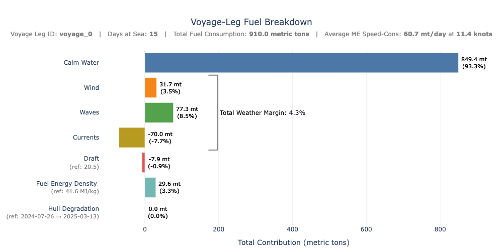
2.4) Advanced Visual: Daily Fuel Breakdown
This plot displays daily fuel consumption as a stacked bar chart, starting with calm water consumption at the base and layering the effects of operational and environmental conditions on top. A dashed line and numeric labels indicate total daily fuel consumption.
# advanced visual
from plotly.subplots import make_subplots
import plotly.graph_objects as go
# --- Colors for consistency ---
component_colors = {
'fuel_calm_water': '#4c78a8',
'abs_contrib_wind_speed': '#f58518',
'abs_contrib_wave_height': '#54a24b',
'abs_contrib_current_speed': '#b79a20',
'abs_contrib_draft_avg': '#e45756',
'abs_contrib_fuel_specific_energy': '#72b7b2',
'abs_fouling': '#9d7de5'
}
# --- Legend labels with references ---
draft_info = avg_draft_per_voyage.loc[avg_draft_per_voyage["voyage_id"] == selected_voyage_id]
if not draft_info.empty:
draft_mode = draft_info.iloc[0]["draft_mode"]
draft_ref_value = (
ballast_draft
if draft_mode == "ballast"
else round(draft_info.iloc[0]["avg_draft_avg"], 1)
)
draft_label = (
"Draft<br>"
f"<span style='font-size:11px; color:gray'>(ref: {draft_ref_value})</span>"
)
else:
draft_label = "Draft"
ballast_draft = ship_info.get("ballast_draft")
lcv_label = "Fuel Energy Density <br><span style='font-size:11px; color:gray'>(ref: 41.6 MJ/kg)</span>"
# Get benchmark info
model_url = f"https://api.toqua.ai/ships/{IMO_NUMBER}/models/latest/metadata"
model_response = requests.get(model_url, headers=headers)
benchmark_label = "Hull Degradation"
if model_response.ok:
model_info = model_response.json()
periods = model_info.get("periods", [])
bm = next((p for p in periods if p.get("type") == "benchmark"), None)
if bm and bm.get("start_date") and bm.get("end_date"):
start = bm["start_date"][:10]
end = bm["end_date"][:10]
benchmark_label = ("Hull Degradation<br>"
f"<span style='font-size:11px; color:gray'>(ref: {start} → {end})</span>"
)
else:
raise Exception(f"❌ API Error {model_response.status_code}: {model_response.text}")
legend_labels = {
'fuel_calm_water': 'Calm Water',
'abs_contrib_wind_speed': 'Wind',
'abs_contrib_wave_height': 'Waves',
'abs_contrib_current_speed': 'Currents',
'abs_contrib_draft_avg': draft_label,
'abs_contrib_fuel_specific_energy': lcv_label,
'abs_fouling': benchmark_label
}
fig = make_subplots(
rows=1, cols=1,
subplot_titles=("Fuel Consumption Over Time",),
specs=[[{"type": "bar"}]]
)
plot_order = fuel_components[::-1]
base_component = 'fuel_calm_water'
adjustment_components = [col for col in plot_order if col != base_component]
stacked_columns = [base_component] + adjustment_components
df_voyage['total_visible_bar'] = df_voyage[stacked_columns].sum(axis=1)
# -- Plot base (calm water) --
fig.add_trace(go.Bar(
x=df_voyage.index,
y=df_voyage[base_component],
name=legend_labels.get(base_component, base_component),
marker_color=component_colors.get(base_component, '#999999'),
hoverinfo='x+y+name'
), row=1, col=1)
# -- Plot adjustment components stacked --
for col in adjustment_components:
fig.add_trace(go.Bar(
x=df_voyage.index,
y=df_voyage[col],
name=legend_labels.get(col, col),
marker_color=component_colors.get(col, '#999999'),
hoverinfo='x+y+name'
), row=1, col=1)
# -- Total fuel dashed line --
fig.add_trace(go.Scatter(
x=df_voyage.index,
y=df_voyage['total_visible_bar'],
mode='lines+markers',
name='Total Fuel',
line=dict(color='black', width=2, dash='dash'),
marker=dict(size=6),
hoverinfo='x+y'
), row=1, col=1)
df_voyage['bar_top'] = (df_voyage[base_component] + df_voyage[adjustment_components].clip(lower=0).sum(axis=1))
# -- Text annotations above bars --
fig.add_trace(go.Scatter(
x=df_voyage.index,
y=df_voyage['bar_top'] + 0.5,
mode='text',
text=[f"{val:.1f} mt" for val in df_voyage['total_visible_bar']],
textposition='top center',
textfont=dict(size=11, color='black', family='Arial Black'),
showlegend=False,
hoverinfo='skip'
), row=1, col=1)
# -- Layout --
avg_fuel_per_day = total_fuel / total_days if total_days else 0
avg_speed = df_voyage['sog'].mean()
fig.update_layout(
barmode='relative',
height=500,
width=1200,
template='plotly_white',
title=dict(
text=(
f'Voyage-leg Fuel Breakdown<br>'
f'<span style="font-size:12px; color:gray">'
f'Voyage Leg ID: <b>{selected_voyage_id}</b> | '
f'Days at Sea: <b>{total_days}</b> | '
f'Total Fuel Consumption: <b>{total_fuel:.1f} metric tons</b> | '
f'Average Speed-Cons: <b>{avg_fuel_per_day:.1f} mt/day</b> at <b>{avg_speed:.1f} knots</b>'
f'</span>'),
x=0.5,
xanchor='center'
),
legend_title=None,
legend=dict(orientation='h',yanchor='bottom',y=-0.45,xanchor='center',x=0.5,font=dict(size=12),title=None),
xaxis_title='Date',
yaxis_title='Fuel Consumption (metric_tons/day)',
margin=dict(t=100, l=30, r=30, b=20)
)
fig.show()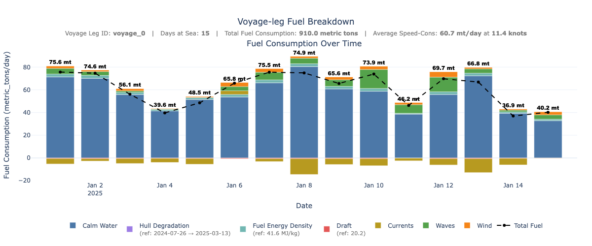
2.5) Combined Standard & Advanced Visuals
The code below generates a two-panel visualization of fuel consumption decomposition for a specific vessel voyage, using Plotly. It first assigns consistent colors and human-readable labels to each fuel component (e.g., wind, waves, current). These labels are dynamically enhanced with metadata from Toqua’s API:
from plotly.subplots import make_subplots
import plotly.graph_objects as go
# -------------------------------
# Define colors for consistency
# -------------------------------
component_colors = {
'fuel_calm_water': '#4c78a8',
'abs_contrib_wind_speed': '#f58518',
'abs_contrib_wave_height': '#54a24b',
'abs_contrib_current_speed': '#b79a20',
'abs_contrib_draft_avg': '#e45756',
'abs_contrib_fuel_specific_energy': '#72b7b2',
'abs_fouling': '#9d7de5'
}
# Reference draft
draft_info = avg_draft_per_voyage.loc[avg_draft_per_voyage["voyage_id"] == selected_voyage_id]
if not draft_info.empty:
draft_mode = draft_info.iloc[0]["draft_mode"]
draft_ref_value = (
ballast_draft
if draft_mode == "ballast"
else round(draft_info.iloc[0]["avg_draft_avg"], 1)
)
draft_label = (
"Draft<br>"
f"<span style='font-size:11px; color:gray'>(ref: {draft_ref_value})</span>"
)
else:
draft_label = "Draft"
# Get benchmark info
model_url = f"https://api.toqua.ai/ships/{IMO_NUMBER}/models/latest/metadata"
model_response = requests.get(model_url, headers=headers)
benchmark_label = "Hull Degradation"
if model_response.ok:
model_info = model_response.json()
periods = model_info.get("periods", [])
bm = next((p for p in periods if p.get("type") == "benchmark"), None)
if bm and bm.get("start_date") and bm.get("end_date"):
start = bm["start_date"][:10]
end = bm["end_date"][:10]
benchmark_label = f"Hull Degradation (ref: {start} → {end})"
else:
raise Exception(f"❌ API Error {model_response.status_code}: {model_response.text}")
# reference lcv
lcv_label = "Fuel Energy Density <br><span style='font-size:11px; color:gray'>(ref: 41.6 MJ/kg)</span>"
# Set final legend labels
legend_labels = {
'fuel_calm_water': 'Calm Water',
'abs_contrib_wind_speed': 'Wind',
'abs_contrib_wave_height': 'Waves',
'abs_contrib_current_speed': 'Current',
'abs_contrib_draft_avg': draft_label,
'abs_contrib_fuel_specific_energy': lcv_label,
'abs_fouling': benchmark_label
}
plot_order = fuel_components[::-1] # bottom to top stack
# -------------------------------
# Split data into + and - parts
# -------------------------------
df_pos = df_voyage[plot_order].clip(lower=0)
df_neg = df_voyage[plot_order].clip(upper=0)
component_totals = df_voyage[fuel_components].sum().sort_values()
# -------------------------------
# Create subplot layout
# -------------------------------
fig = make_subplots(
rows=1, cols=2,
column_widths=[0.55, 0.45],
subplot_titles=("Fuel Consumption Over Time", "Contribution by Factor"),
specs=[[{"type": "bar"}, {"type": "bar"}]]
)
# -------------------------------
# Left plot: Stacked bar over time
# -------------------------------
base_component = 'fuel_calm_water'
adjustment_components = [col for col in plot_order if col != base_component]
stacked_columns = [base_component] + adjustment_components
df_voyage['total_visible_bar'] = df_voyage[stacked_columns].sum(axis=1)
# Plot calm water baseline
fig.add_trace(go.Bar(
x=df_voyage.index,
y=df_voyage[base_component],
name=legend_labels.get(base_component, base_component),
marker_color=component_colors.get(base_component, '#999999'),
hoverinfo='x+y+name'
), row=1, col=1)
# Plot all adjustment components stacked on top
for col in adjustment_components:
fig.add_trace(go.Bar(
x=df_voyage.index,
y=df_voyage[col],
name=legend_labels.get(col, col),
marker_color=component_colors.get(col, '#999999'),
hoverinfo='x+y+name'
), row=1, col=1)
# Compute total bar height for each day
df_voyage['bar_top'] = (df_voyage[base_component] + df_voyage[adjustment_components].clip(lower=0).sum(axis=1))
# Add dashed black line for total fuel
fig.add_trace(go.Scatter(
x=df_voyage.index,
y=df_voyage['total_visible_bar'],
mode='lines+markers',
name='Total Fuel',
line=dict(color='black', width=2, dash='dash'),
marker=dict(size=6),
hoverinfo='x+y'
), row=1, col=1)
# Add total fuel value as text just above the bar
fig.add_trace(go.Scatter(
x=df_voyage.index,
y=df_voyage['bar_top'] + 0.5, # minimal lift for readability
mode='text',
text=[f"{val:.1f} mt" for val in df_voyage['total_visible_bar']],
textposition='top center',
textfont=dict(
size=11,
color='black',
family='Arial Black'
),
showlegend=False,
hoverinfo='skip'
), row=1, col=1)
# -------------------------------
# Right plot: Horizontal breakdown with ordering + annotation
# -------------------------------
component_totals = df_voyage[fuel_components].sum()
# Reorder: Calm Water → Weather → Other → Zero
calm_water = ['fuel_calm_water']
weather_order = ['abs_contrib_wind_speed', 'abs_contrib_wave_height', 'abs_contrib_current_speed']
zero_components = component_totals[component_totals == 0].index.tolist()
non_zero_components = [c for c in component_totals.index if c not in zero_components]
non_zero_calm = [c for c in calm_water if c in non_zero_components]
non_zero_weather = [c for c in weather_order if c in non_zero_components]
non_zero_others = [c for c in non_zero_components if c not in non_zero_calm + non_zero_weather]
ordered_components = (
non_zero_calm +
non_zero_weather +
non_zero_others +
[c for c in zero_components if c not in non_zero_calm + non_zero_weather + non_zero_others]
)
component_totals = component_totals.loc[ordered_components]
total_sum = component_totals.sum()
# Build bar + labels
y_labels = [legend_labels.get(col, col) for col in ordered_components]
y_vals = list(range(len(ordered_components)))
for i, col in enumerate(ordered_components):
value = component_totals[col]
pct = (value / total_sum) * 100 if total_sum else 0
text = f"{value:.1f} mt<br>({pct:.1f}%)"
fig.add_trace(go.Bar(
x=[value],
y=[i],
orientation='h',
marker_color=component_colors.get(col, '#999999'),
text=None,
hoverinfo='skip',
showlegend=False,
cliponaxis=False
), row=1, col=2)
fig.add_annotation(
x=max(value, 0) + 5,
y=i,
text=text,
showarrow=False,
font=dict(size=11, color="black"),
xref='x2',
yref='y2',
xanchor='left',
yanchor='middle',
row=1, col=2
)
# Add weather group brace
weather_components = weather_order
weather_indices = [i for i, col in enumerate(ordered_components) if col in weather_components]
if weather_indices:
y_top = max(weather_indices) + 0.5
y_bottom = min(weather_indices) - 0.5
y_mid = (y_top + y_bottom) / 2
weather_bar_max = max([component_totals.get(c, 0) for c in weather_components])
x_offset = weather_bar_max + 120
x_text = x_offset + 5
cap_length = 25
line_color = "gray"
line_width = 2
weather_pct = (component_totals[weather_components].sum() / total_sum) * 100 if total_sum else 0
fig.add_shape(type="line", xref="x2", yref="y2",
x0=x_offset, x1=x_offset,
y0=y_bottom, y1=y_top,
line=dict(color=line_color, width=line_width),
row=1, col=2)
fig.add_shape(type="line", xref="x2", yref="y2",
x0=x_offset, x1=x_offset - cap_length,
y0=y_top, y1=y_top,
line=dict(color=line_color, width=line_width),
row=1, col=2)
fig.add_shape(type="line", xref="x2", yref="y2",
x0=x_offset, x1=x_offset - cap_length,
y0=y_bottom, y1=y_bottom,
line=dict(color=line_color, width=line_width),
row=1, col=2)
fig.add_annotation(
x=x_text,
y=y_mid,
xref='x2',
yref='y2',
text=f"Total Weather Margin: {weather_pct:.1f}%",
showarrow=False,
align='left',
font=dict(size=12, color='black'),
xanchor='left',
yanchor='middle',
row=1, col=2
)
# Fix axis to reverse so Calm Water appears first
fig.update_yaxes(
tickmode='array',
tickvals=y_vals,
ticktext=y_labels,
automargin=True,
autorange='reversed',
row=1, col=2
)
# -------------------------------
# Layout and styling
# -------------------------------
total_days = df_voyage.index.nunique()
total_fuel = df_voyage['total_visible_bar'].sum()
fig.update_layout(
barmode='relative',
height=500,
width=1650,
template='plotly_white',
title= dict(
text=f'Voyage-Leg Fuel Contribution Breakdown Over Time<br>'
f'<span style="font-size:12px; color:gray">'
f'Voyage Leg ID: <b>{selected_voyage_id}</b> | '
f'Days at Sea: <b>{total_days}</b> | '
f'Total Fuel Consumption: <b>{total_fuel:.1f} metric tons</b>'
f'</span>',
x=0.5,
xanchor='center'
),
legend_title= None,
legend=dict(orientation='h',yanchor='bottom', y=-0.45, xanchor='center', x=0.5),
xaxis_title='Date',
yaxis_title='Fuel Consumption (metric_tons/day)',
xaxis2=dict(title='Total Contribution (metric_tons)', showgrid=True, zeroline=True, tickformat=".0f"),
yaxis2=dict(automargin=True, showticklabels=False),
margin=dict(t=100, l=30, r=30, b=10)
)
fig.show()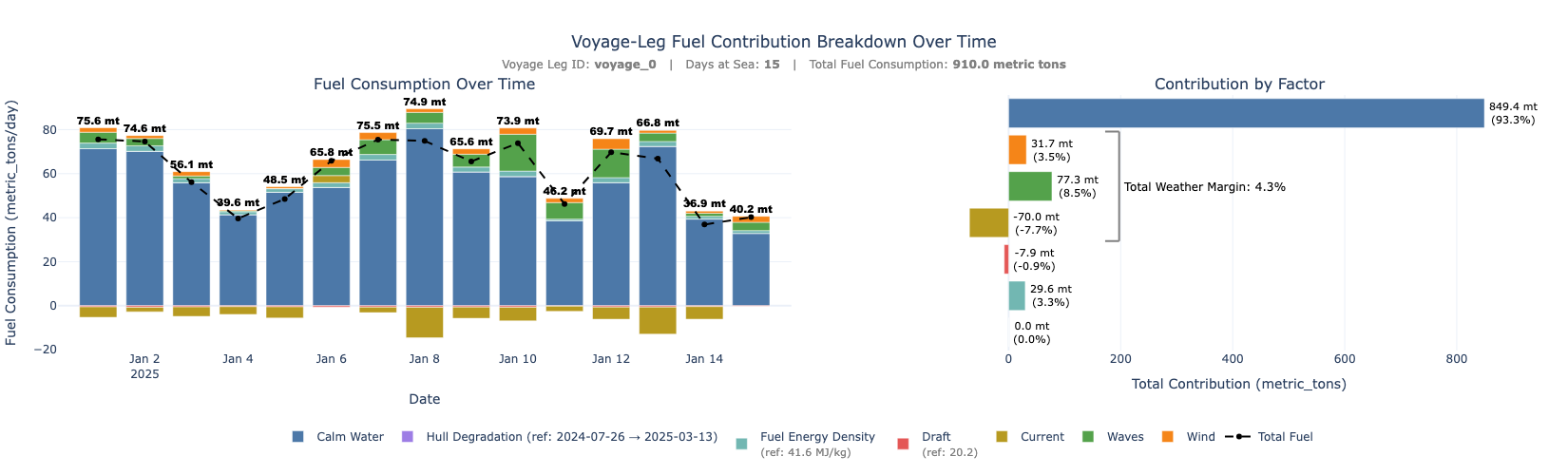
Updated 10 months ago